Complexity Basics and Segment Trees
Slides covered: 29–44
Topic folder: 01 Foundations
Fast take
- Separate preprocessing, query, and storage. Geometric search algorithms are usually judged by all three.
- Also separate single-shot from repetitive-mode and counting from reporting.
- Reporting problems are often output-sensitive, so query time becomes O(log N + K) or similar.
- A segment tree stores intervals via a canonical decomposition into O(log N) standard intervals.
Recording notes
Recording references: CS 564 - 01.23 1.1.txt, CS 564 - 01.30 3.1.txt
- The lecture kept coming back to the same practical question: are you paying preprocessing for one query or for many queries? That choice changes the whole design.
- Normalization here is basically rank-based coordinate compression. It is boring but useful, like most things humans try to ignore until implementation time.
- For segment trees, the important fact is not the picture but the guarantee that one interval is allocated to only O(log N) nodes.
- Do not blur counting and reporting. Listing objects can dominate the runtime even if search itself is logarithmic.
Motivation
This file explains how geometric algorithms are measured, what counting versus reporting means, and why preprocessing matters. It also introduces the segment tree, a basic data structure used later.
Lecture Roadmap
- Know the problem definition.
- Know the main geometric idea.
- Know the key data structure or primitive test.
- Know the preprocessing / query / storage or total running time.
- Know one small example by hand.
Detailed lecture notes
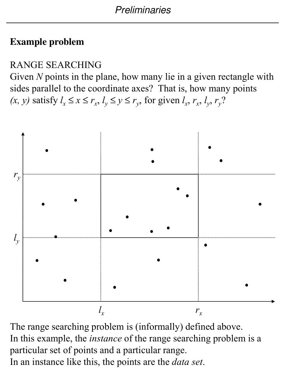
Slide 29: Range searching (informal)
Problem: Given \(N\) points in the plane, how many lie in an axis-aligned rectangle? That is, how many \((x,y)\) satisfy
for given \(\ell_x, r_x, \ell_y, r_y\)?
An instance consists of the point set and the query rectangle (the points are the data set).
Slide 30: Model of computation
We want efficient algorithms; cost is a function of instance size \(N\).
We use an abstract real RAM (random-access machine), a slight variant of the model in Aho et al. (1974). Unit-cost primitives include:
- Arithmetic: \(+, -, \times, /\)
- Comparisons: \(<, \le, =, \neq, \ge, >\)
- Memory access
- Analytic functions: roots, trig, exp, log
Numbers are reals with infinite precision (idealized vs. actual hardware).
Slide 31: Asymptotic notation
We measure time and memory as functions of input size \(N\).
| Notation | Meaning (intuitive) |
|---|---|
| \(O(f(N))\) (upper / worst-case bound) | \(g(N) \le C f(N)\) for large \(N\), some constant \(C > 0\) |
| \(\Omega(f(N))\) (lower bound) | \(g(N) \ge C f(N)\) for large \(N\) |
| \(\Theta(f(N))\) (tight) | \(C_1 f(N) \le g(N) \le C_2 f(N)\) for large \(N\) |
Notes:
- These denote sets of functions; one writes \(f(N) \in O(\log N)\) (the slides also use “\(=\)” informally).
- Dominant terms control growth, e.g. \(4N + 20\log N + 100 \in O(N)\).
- Most discussion emphasizes worst-case bounds.
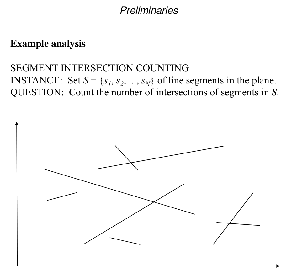
Slide 32–33: Segment intersection counting
INSTANCE: A set \(S = \{s_1, s_2, \ldots, s_N\}\) of line segments in the plane.
QUESTION: Count how many pairs of distinct segments intersect.
Naive algorithm (conceptual):
count ← 0
for i = 1 to N
  for j = 1 to N
    if i ≠ j and s_i ∩ s_j ≠ ∅ then count ← count + 1
output count
- Storage: \(O(N)\) for \(S\)
- Time: \(O(N^2)\) nested loops
- Assumes a primitive segment–segment intersection test.
Slide 34: Preprocessing, query, storage; modes
- Preprocessing — One-time cost to organize the data (often into a structure).
- Query — Cost to answer one query against that structure.
- Storage — Memory for static/dynamic structures.
Single-shot: one data set, one query — often best to scan in \(O(N)\) time, \(O(N)\) space, no preprocessing.
Repetitive mode: one data set, many queries — we may pay preprocessing to make each query faster than \(O(N)\).
Slide 35: Counting vs. reporting
Reporting — List all objects satisfying the query.
Range searching (formal instance):
- INSTANCE: Point set \(S = \{p_1,\ldots,p_N\}\), \(p_i = (x_i,y_i)\), and axis-aligned rectangle \(R = [\ell_x, r_x] \times [\ell_y, r_y]\).
- QUESTION (counting): How many points of \(S\) lie in \(R\)?
- QUESTION (reporting): Which points lie in \(R\)?
Slide 36: Output-sensitive complexity
Interval enclosure example
- INSTANCE: Points \(S = \{x_1,\ldots,x_N\}\) on the real line and query interval \(Q = [\ell, r]\).
- QUESTION: Which points satisfy \(\ell \le x_i \le r\)?
Repetitive-mode approach:
- Preprocessing: Sort \(S\) into array \(A\) — \(O(N \log N)\).
- Query: Binary search for lower bound \(\ge \ell\) and upper bound \(\le r\) — \(O(\log N)\) each.
- Report all points in the index range — \(O(K)\) if \(K\) points are reported.
So query time is \(O(\log N + K)\) when reporting matters; without listing output, counting can be \(O(\log N)\).
Slide 37: Other cost notions
- Preprocessing cost — Trade-offs between space, preprocessing time, and query time.
- Amortized cost — Average over mixes of cheap and expensive operations.
- Normalization — Map coordinates into \([1,N]\) by rank order. Usually \(O(N \log N)\) preprocessing sort and \(O(\log N)\) rank lookup per query when needed.
Slide 38: Segment tree setup
Consider intervals on the real line whose endpoints come from a fixed set of \(N\) abscissae. The segment tree for scope \([\ell, r]\) is a fixed tree shape; intervals are stored in auxiliary structures at nodes.
Assume WLOG endpoints are normalized to \(\{1,\ldots,N\}\) and the tree is built for scope \([1,N]\).
Node \(v\) stores:
| Field | Meaning |
|---|---|
| \(B(v)\) | Start of \(v\)’s scope interval |
| \(E(v)\) | End of \(v\)’s scope interval |
| \(Lchild(v)\) | Left child = subtree over \([B(v), \lfloor(B(v)+E(v))/2\rfloor]\) |
| \(Rchild(v)\) | Right child (upper half-interval) |
Notation: \(T(\ell,r)\) = segment tree over scope \([\ell,r]\).
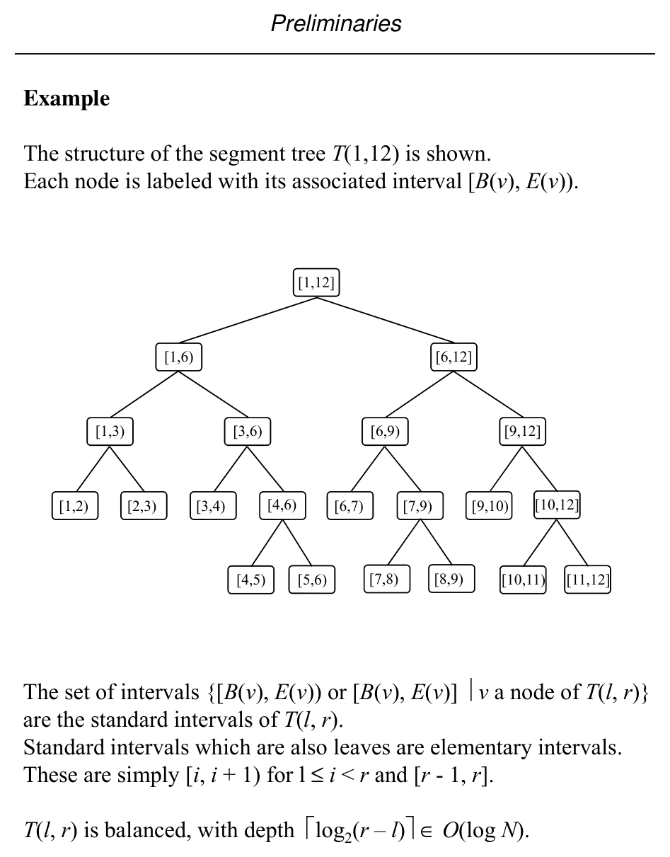
Slide 39: Example \(T(1,12)\)
Each node is labeled with its associated half-open interval \([B(v), E(v))\) (see figure).
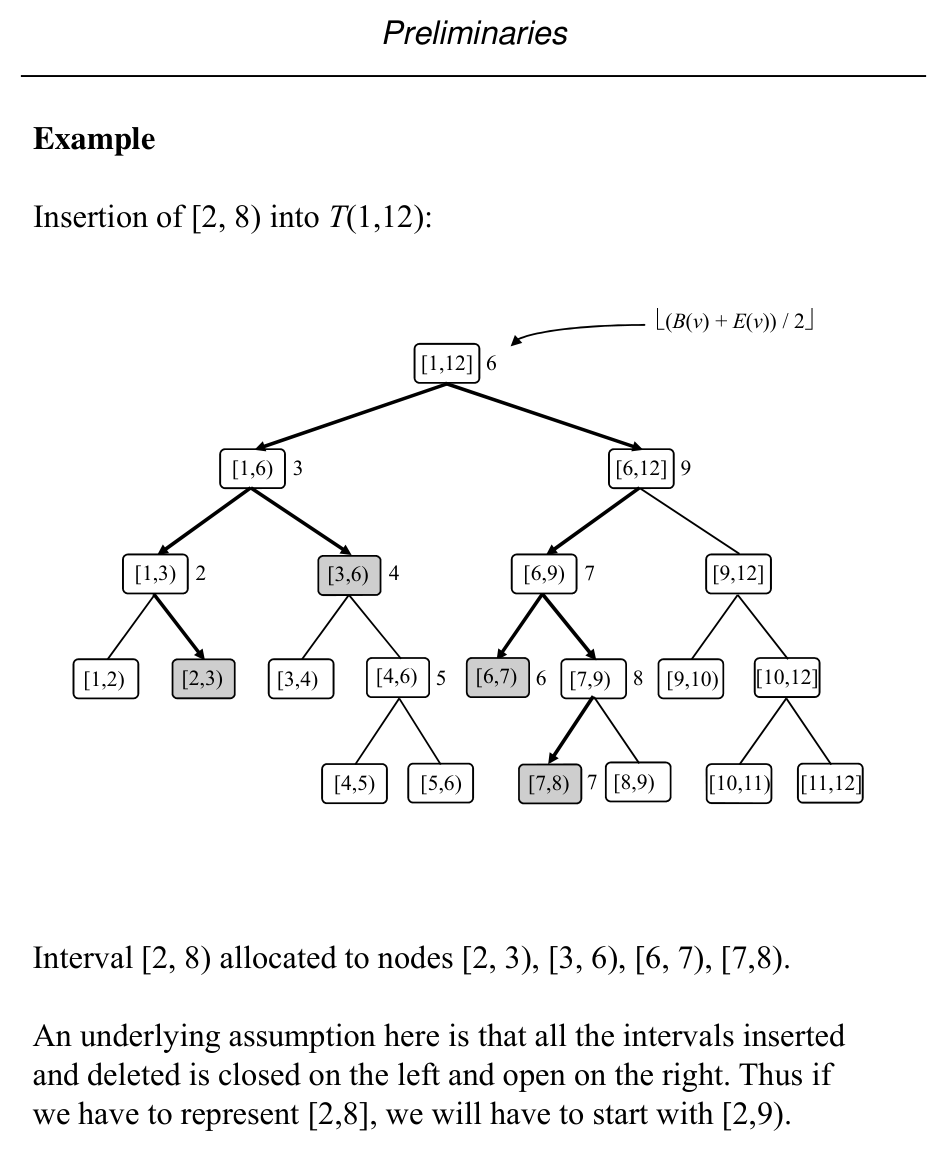
Slide 40: Inserting an interval
Intervals with endpoints in \(\{\ell,\ell+1,\ldots,r\}\) can be maintained so insertion/deletion runs in \(O(\log N)\) per operation (per slide).
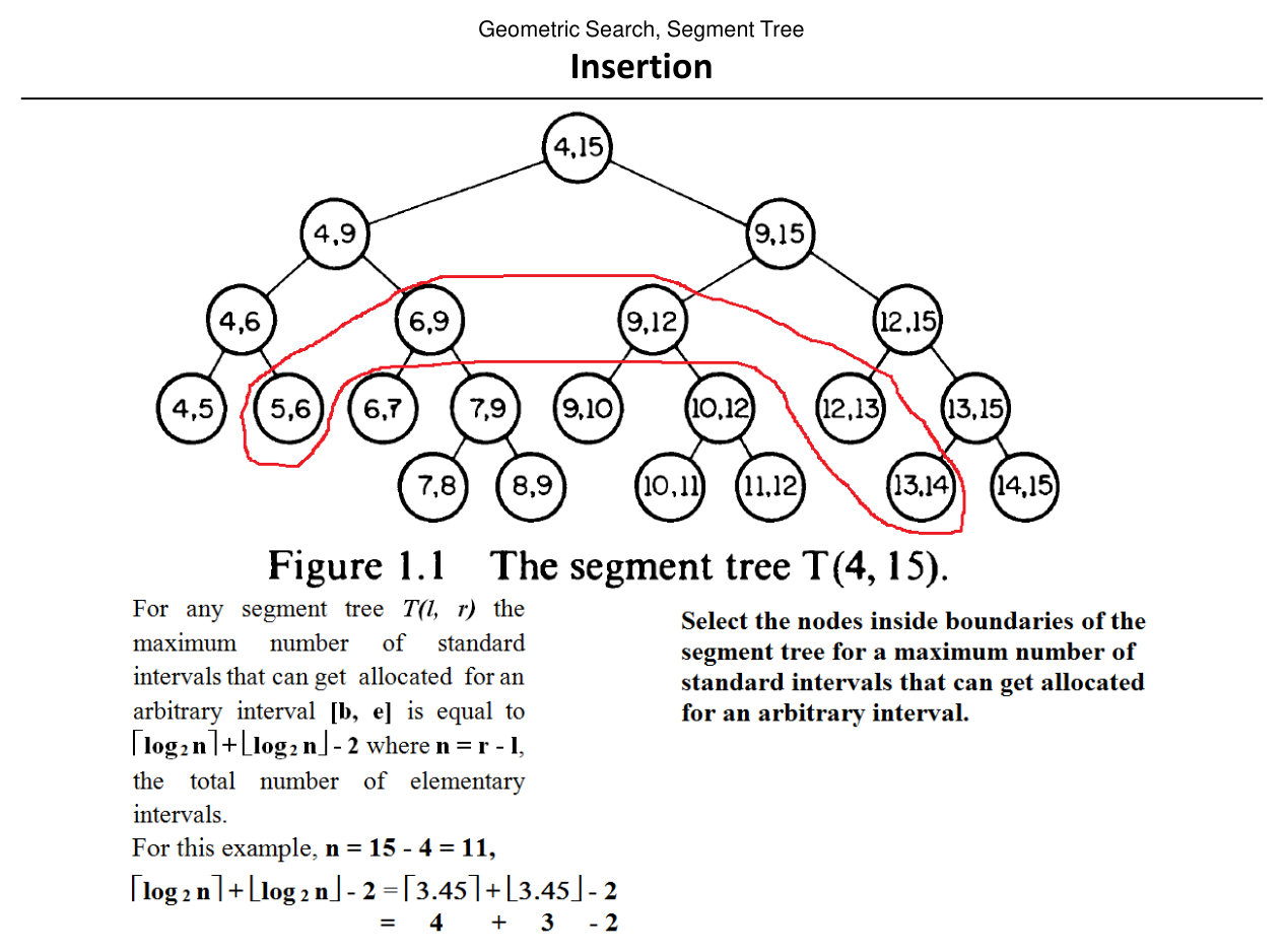
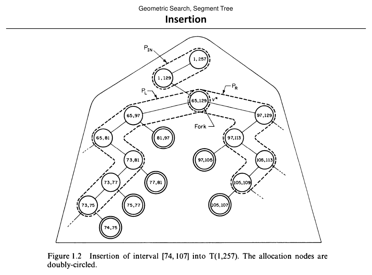
For \(r - \ell > 3\), an interval \([b,e]\) is partitioned into standard (canonical) node intervals; the number of pieces is \(O(\log N)\).
InsertSegmentTree(b, e, v) (sketch):
- If \([B(v),E(v))\) is fully covered by \([b,e]\), attach the interval to \(A(v)\) and return.
- Else, if \(b < \lfloor(B(v)+E(v))/2\rfloor\), recurse on \(Lchild(v)\).
- If \(\lfloor(B(v)+E(v))/2\rfloor < e\), recurse on \(Rchild(v)\).
Slide 41: Structure after insertions
Illustration of \(T(1,12)\) with midpoint splits \(\lfloor(B(v)+E(v))/2\rfloor\) at internal nodes (see figure).
Slide 42–43: Insertion figures
Slide 44: Deleting an interval
DeleteSegmentTree(b, e, v) mirrors insertion: if \([B(v),E(v))\) is fully inside \([b,e]\), remove the interval from \(A(v)\); otherwise recurse to children as in insertion.
Recap
- Asymptotics: \(O\), \(\Omega\), \(\Theta\) describe worst-case, lower, and tight bounds as \(N \to \infty\); they are sets of functions (informally written with “\(=\)”).
- Cost models: Real RAM with unit-cost arithmetic, comparisons, memory, and analytic primitives; use these to state preprocessing, query, and storage separately.
- Modes: Single-shot vs. repetitive; counting vs. reporting; output-sensitive bounds like \(O(\log N + K)\) when listing \(K\) objects.
- Segment tree: Built on a fixed scope interval \([\ell,r]\); each node stores a sub-interval \([B(v),E(v))\); intervals are canonical into \(O(\log N)\) nodes; insert/delete walk the tree in \(O(\log N)\) per update.