Graham’s Scan

Slides covered: 206–219

Topic folder: 03 Convex Hulls

Fast take

• Pick an interior reference point, sort by polar order, then scan and delete non-left turns.
• Orientation replaces expensive angle computation whenever possible.
• The scan phase is linear after sorting, so total time is O(N log N).
• Collinear middle points must be removed because they are not hull vertices.

Recording notes

Recording references: CS 564 - 02.25 10.1.txt

• The lecture emphasized that the real trick is not sorting by angle itself, but comparing order with left-turn tests instead of trig.
• Backtracking is the mechanism that repairs local mistakes as the scan moves forward.
• This is worst-case optimal in 2D, but it is still a static planar algorithm, not the universal answer to everything.
• If you only memorize the pseudocode and miss why non-left turns are deleted, you missed the algorithm.

Motivation

Graham’s scan sorts points around a reference point and then removes right turns while scanning. It is one of the classic optimal planar convex hull algorithms.

Lecture Roadmap

• Know the problem definition.
• Know the main geometric idea.
• Know the key data structure or primitive test.
• Know the preprocessing / query / storage or total running time.
• Know one small example by hand.

Detailed lecture notes

Slide 206: Concept

A point inside a triangle determined by three points of \(S\) cannot be a vertex of \(H(S)\). A naive approach tests many triangles per point.

Graham’s scan (1972) answers “is \(p\) inside some triangle of \(S\)?” more efficiently. Idea: if \(p\) is not a hull vertex, then \(p\) lies in some triangle \(O p_1 p_2\) with \(O\) interior and \(p_1,p_2\) hull vertices — the algorithm discovers this during a scan.

The algorithm has preparation and scan phases; it is a single-shot method (one hull for a given \(S\)).

Slide 207: Centroid and lexicographic sort

The centroid of points \(p_1,\ldots,p_N\) is their arithmetic mean \(\frac{1}{N}\sum_i p_i\) (coordinate-wise).

Lexicographic sort — Sort objects by a primary key; ties broken by secondary key, then tertiary, etc. (e.g. English words: “farther / faster / fastest / father”).

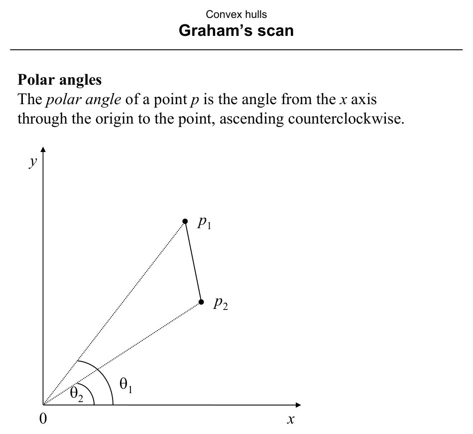
Slide 208: Polar angles

The polar angle of point \(p\) is the angle from the \(x\)-axis through the origin to \(p\), measured counterclockwise.

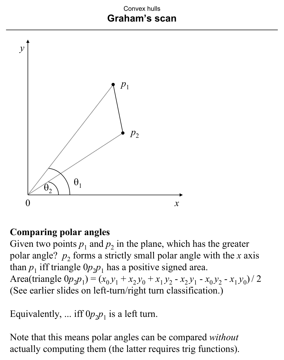
Slide 209: Comparing polar angles without trig

For two points \(p_1, p_2\), point \(p_2\) has smaller polar angle than \(p_1\) iff triangle \(0\, p_2\, p_1\) has positive signed area:

\[ \text{Area}(\triangle 0 p_2 p_1) = \frac{1}{2}\bigl(x_0 y_1 + x_2 y_0 + x_1 y_2 - x_2 y_1 - x_0 y_2 - x_1 y_0\bigr) \]

(with origin as \(p_0=(0,0)\) in the usual embedding) — equivalently a left-turn test. So polar order is compared using orientation, not \(\arctan\).

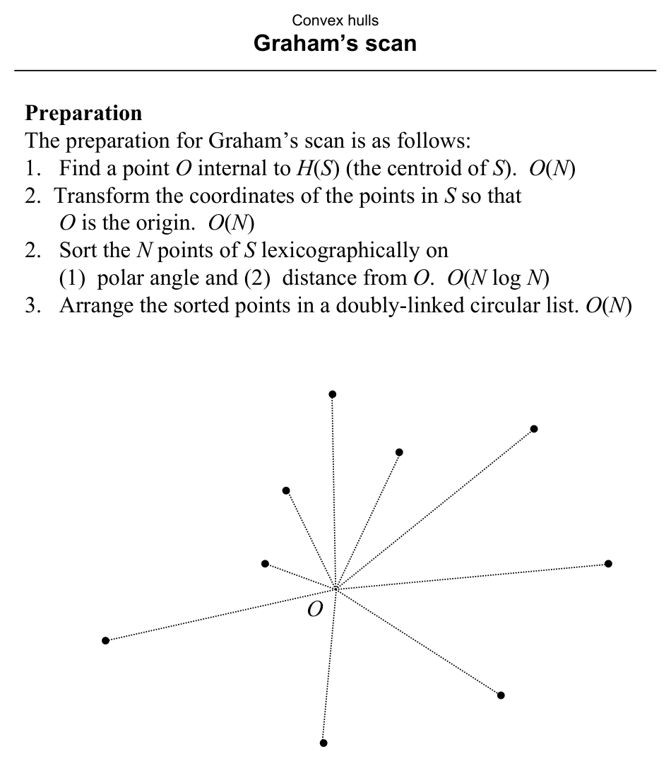
Slide 210: Preparation

1. Find \(O\) strictly inside \(H(S)\) (e.g. centroid of \(S\)) — \(O(N)\).
2. Translate so \(O\) is the origin — \(O(N)\).
3. Sort the \(N\) points lexicographically by (polar angle, then distance from \(O\)) — \(O(N \log N)\).
4. Build a doubly-linked circular list of sorted points — \(O(N)\).

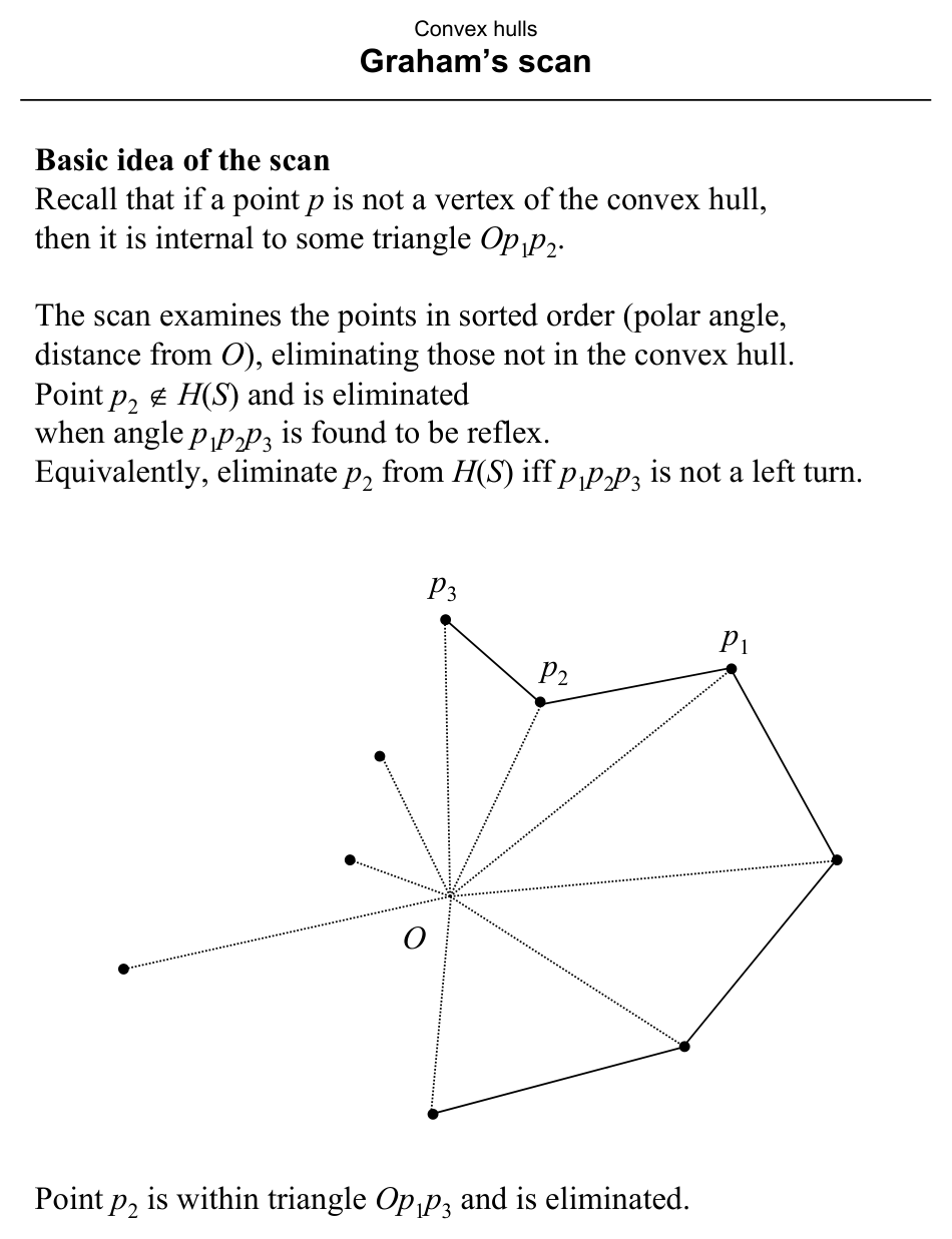
Slide 211: Scan idea

Points are examined in sorted order. A point \(p_2\) not on \(H(S)\) lies inside some triangle \(O p_1 p_3\) and is removed when the turn \(\angle p_1 p_2 p_3\) is reflex — equivalently, eliminate \(p_2\) iff \(p_1 p_2 p_3\) is not a left turn. Collinear middle points are eliminated as non-extreme.

Slide 212: Informal scan

Start at START = rightmost point of minimum \(y\) (a hull vertex). Repeatedly examine consecutive triples \(p_1,p_2,p_3\):

• If right turn, delete \(p_2\) and backtrack to test \(p_0,p_1,p_3\).
• If left turn, advance.
• Collinear: eliminate \(p_2\).

Scan ends when it wraps to START again. START is never deleted; backtracking does not go past START’s predecessor.

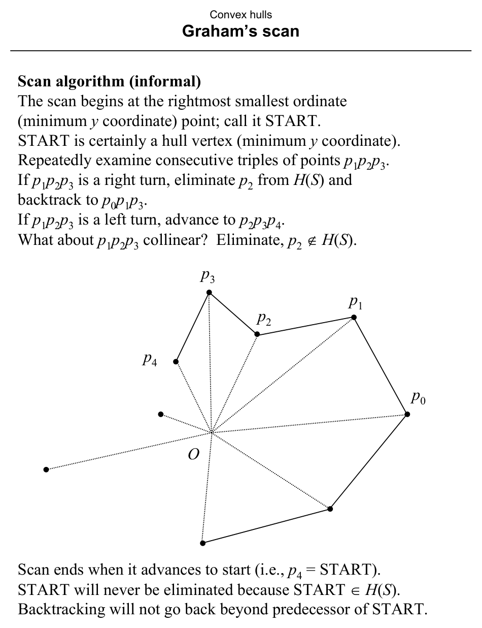
Slide 213: Backtracking

Multiple backtracks in a row may delete a chain of points. Backtracking always terminates at START. No point is deleted more than once.

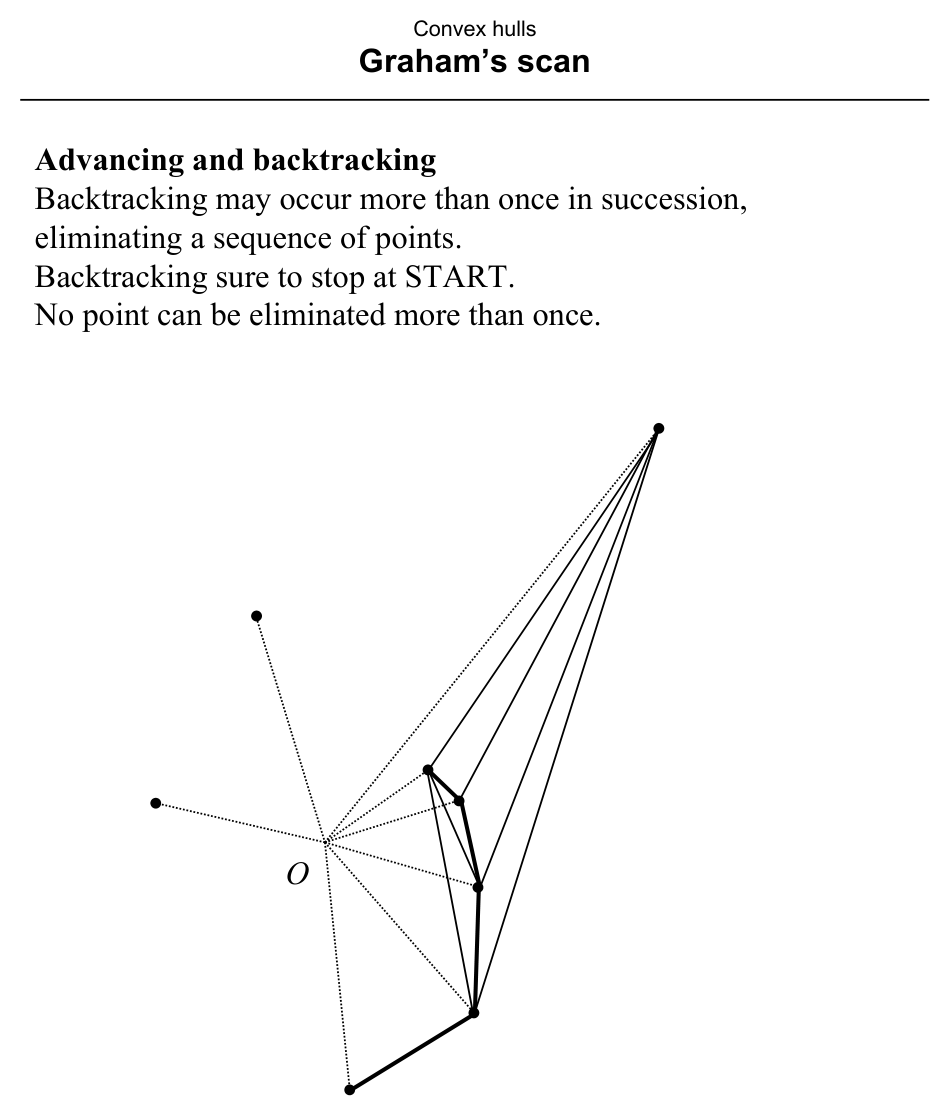
Slide 214: Algorithm (Preparata, p. 108)

1. Find interior point \(O\).
2. With \(O\) as origin, sort \(S\) lexicographically by (polar angle, distance from \(O\)). Build a circular doubly-linked list with pointers NEXT, PRED, and pointer START.

Scan:

v ← START
w ← PRED[v]          /* point just before START */
f ← false            /* true once we've wrapped */
while NEXT[v] ≠ START or f = false do
  if NEXT[v] = w then f ← true endif
  if Left(v, NEXT[v], NEXT[NEXT[v]]) then
    v ← NEXT[v]      /* advance */
  else
    delete NEXT[v]   /* O(1) list delete */
    v ← PRED[v]      /* backtrack */
  endif
endwhile

Here Left(·,·,·) is the left-turn (orientation) primitive.

Slide 215: Analysis

• Time: \(O(N \log N)\) — dominated by sorting; the scan is \(O(N)\) (each step advances or backtracks; at most \(O(N)\) advances and \(O(N)\) backtracks).
• Space: \(O(N)\) for the list.

Slide 216: Upper and lower hulls

Split \(S\) by the line through points \(\ell\) and \(r\) with min and max \(x\)-coordinate. The line partitions remaining points into upper and lower subsets (each includes \(\ell,r\)). Each subset forms an \(x\)-monotone chain; concatenating lower and upper chains yields \(H(S)\).

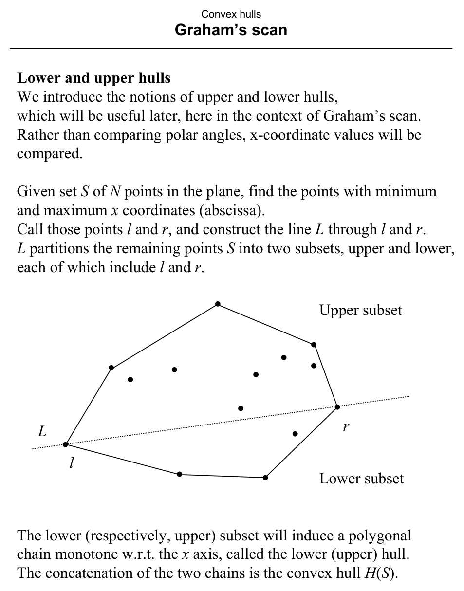
Slide 217: Upper hull

Sort the upper subset by decreasing \(x\). Apply Graham scan from \(r\) to \(\ell\). This matches the general method with reference “at \((0,-\infty)\)” so decreasing \(x\) corresponds to increasing polar angle.

(Text p. 109 erratum: says “increasing” but should be decreasing.)

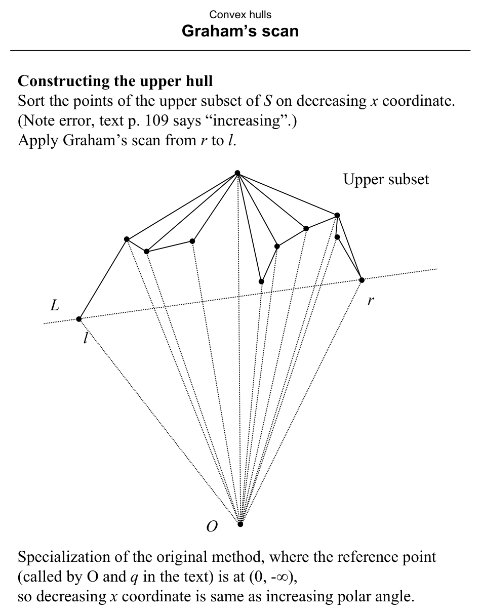
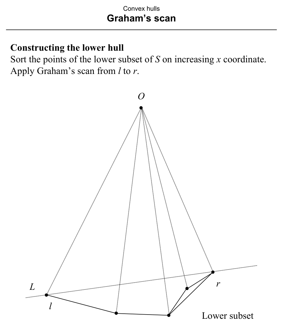
Slide 218: Lower hull

Sort the lower subset by increasing \(x\). Graham scan from \(\ell\) to \(r\).

Slide 219: Summary

• \(O(N \log N)\) is worst-case optimal for the planar hull in the algebraic decision-tree model tied to sorting.
• Further algorithms are still useful for: expected-case behavior, \(d>2\), dynamic settings, parallel structure, and additional insights.

Recap

• Preparation: interior point \(O\) (often centroid), sort by (polar angle, distance) from \(O\), doubly-linked cyclic list; polar order compared via orientation, not trig.
• Scan: walk the sorted cycle; on a non-left turn at \(p_1,p_2,p_3\), delete \(p_2\) and backtrack; only \(O(N)\) advances/backtracks total after \(O(N \log N)\) sort.
• Overall: \(O(N \log N)\) time, \(O(N)\) space; upper/lower hull variant splits by min/max \(x\) and sorts along monotone chains.
• Why more algorithms later: expected case, \(d>2\), dynamic updates, and parallel structure differ from this static planar scan.