Dynamic Hull Maintenance Under Insertion
Slides covered: 245–263
Topic folder: 03 Convex Hulls
Fast take
- In the insertion-only setting, maintain the hull as points arrive one by one.
- If the new point lies inside the current hull, nothing changes.
- If it lies outside, find the left and right supporting tangents and replace the visible chain.
- Dynamic quality is judged differently: update time matters, not just final total time.
Recording notes
Recording references: CS 564 - 03.04 12.1.txt
- The lecture carefully separated static, dynamic, online, offline, and real-time. Do not merge those words into one fuzzy blob.
- For insertion-only hull maintenance, the essential operation is tangent search from the new point to the current hull.
- Real-time claims only make sense relative to the inter-arrival delay of updates.
- Dynamic algorithms are about maintaining structure under change, not rerunning a static algorithm and pretending that counts as clever.
Motivation
Here the hull is maintained as points arrive one by one. The key task is to find the two supporting vertices from the new point and update the stored hull efficiently.
Lecture Roadmap
- Know the problem definition.
- Know the main geometric idea.
- Know the key data structure or primitive test.
- Know the preprocessing / query / storage or total running time.
- Know one small example by hand.
Detailed lecture notes
Slides 245–246: Dynamic hull under insertion
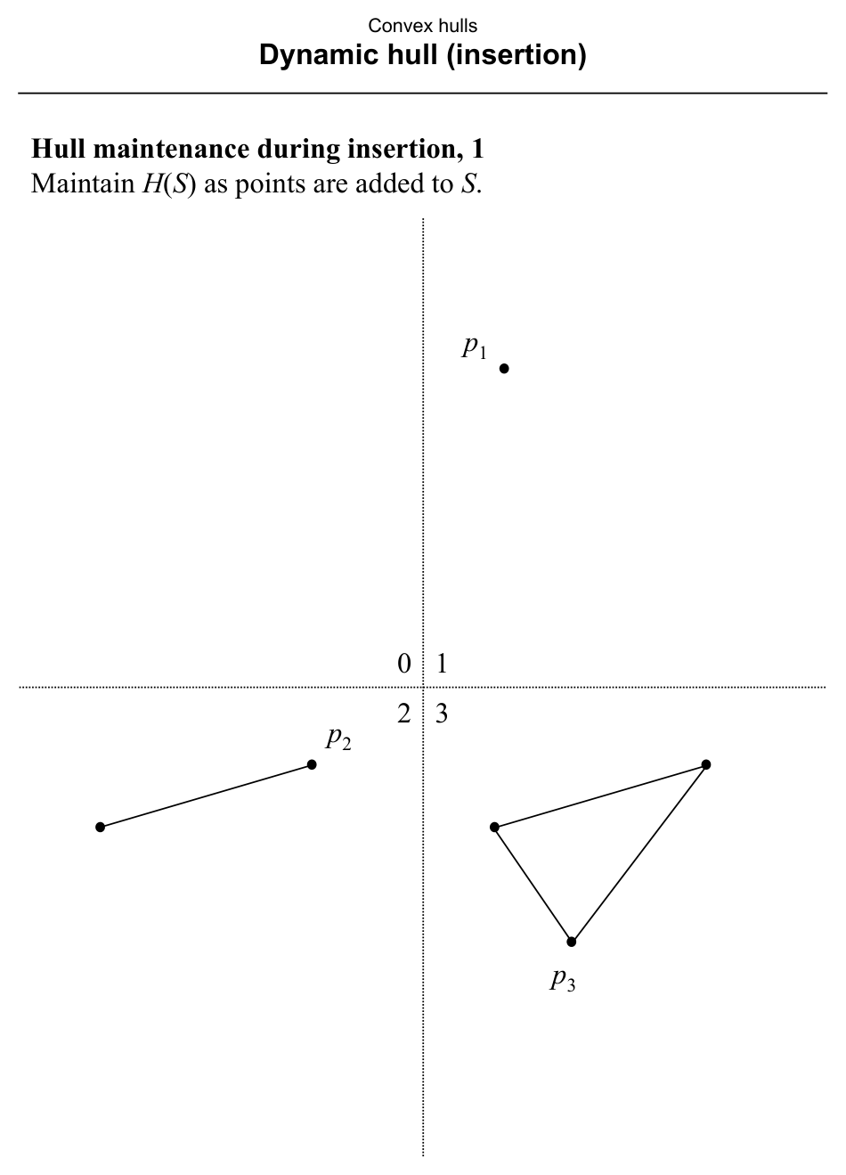
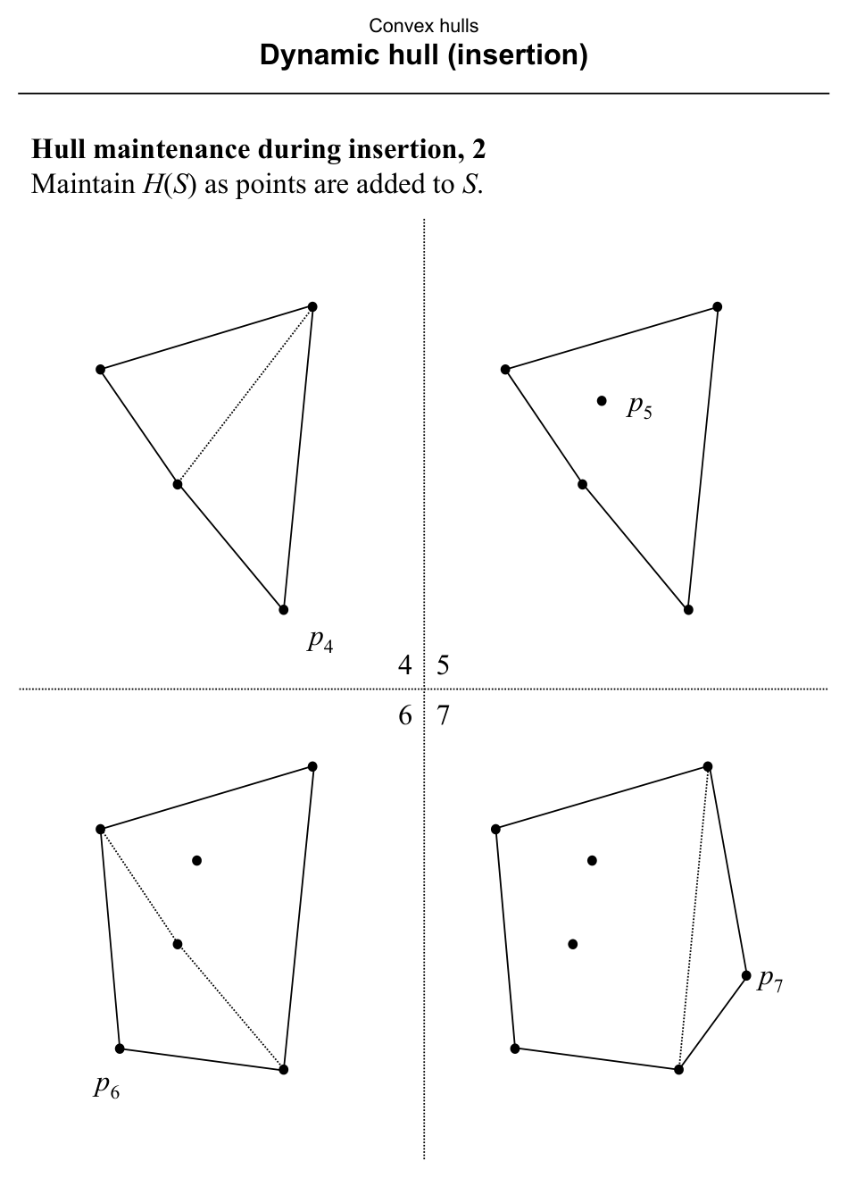
Maintain \(H(S)\) as points are added to \(S\).
Slide 247: Terminology
| Term | Meaning |
|---|---|
| Static | The object set is fixed between operations (e.g. between queries). |
| Dynamic | Insertions/deletions may occur; \(S\) lives in an updatable structure. |
| On-line | No lookahead — each operation must be handled as inputs arrive. |
| Off-line | All data available together (static or batched dynamic). |
| Real-time | Updates must finish within a fixed inter-arrival budget (often \(O(\log N)\)). |
Slide 248: Problem statements
ON-LINE CONVEX HULL
INSTANCE: Sequence \(p_1,\ldots,p_N\) in the plane.
QUESTION: After processing \(p_i\), maintain \(H(\{p_1,\ldots,p_i\})\).
REAL-TIME CONVEX HULL — Same, but with constant delay between arrivals.
DYNAMIC CONVEX HULL (maintenance) — Start from empty \(S\); process a sequence of insertions and deletions (only inserted points may be deleted). Maintain \(H(S)\) throughout.
Slides 245–263 focus on insertion-only on-line/real-time; general dynamic hull is mentioned for later.
Slide 249: Preparata (1979) — key idea 1
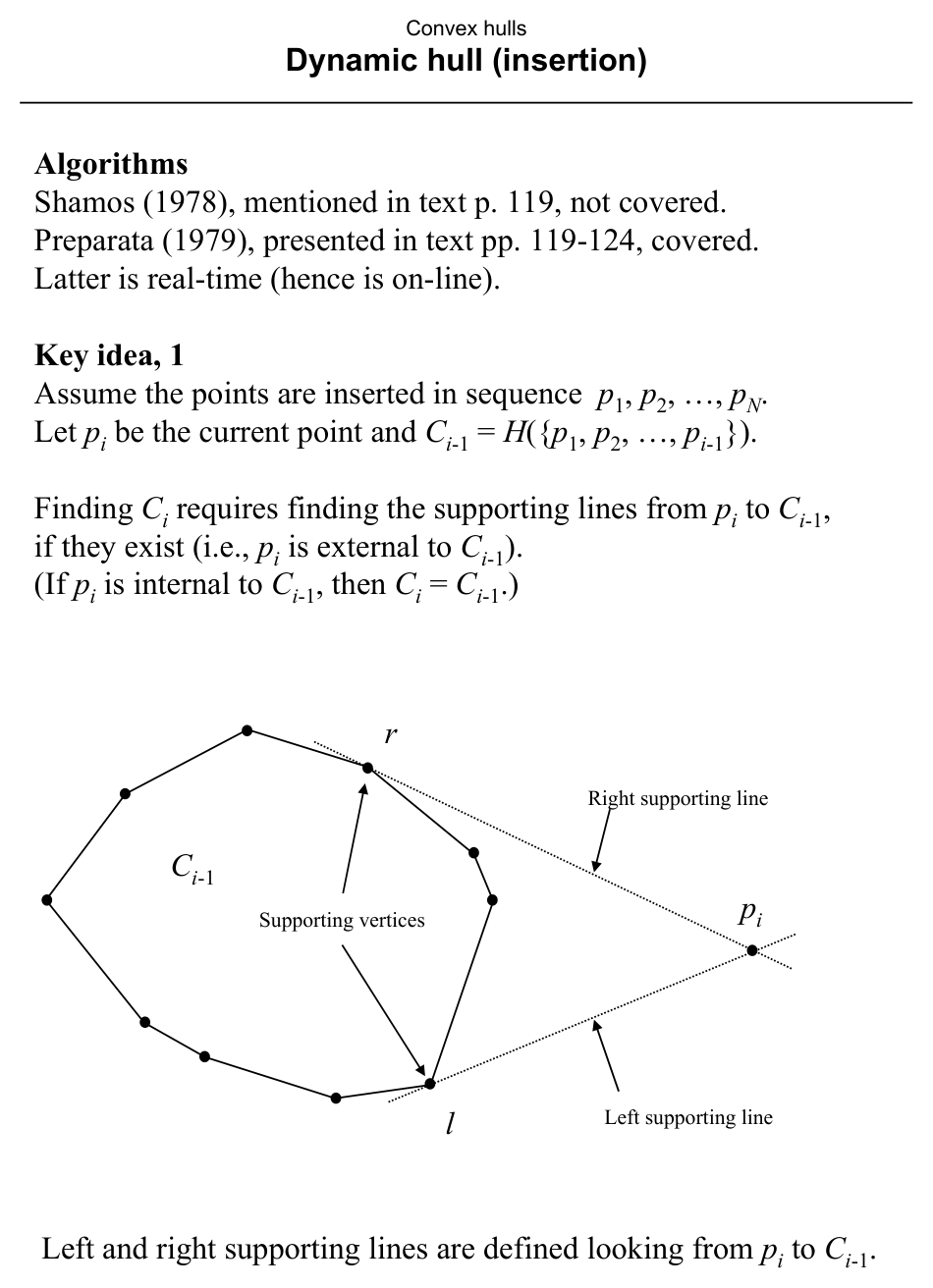
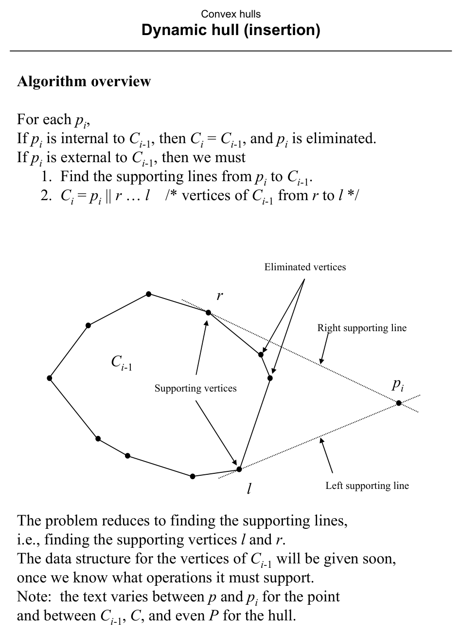
Process insertions \(p_1,\ldots,p_N\). Let \(C_{i-1} = H(\{p_1,\ldots,p_{i-1}\})\) and \(p_i\) be the new point.
- If \(p_i\) is inside \(C_{i-1}\), then \(C_i = C_{i-1}\).
- If \(p_i\) is outside, update requires supporting lines from \(p_i\) to \(C_{i-1}\): left and right supporting vertices \(\ell, r\) (as viewed from \(p_i\) toward \(C_{i-1}\)).
Slide 250: Supporting lines (example)
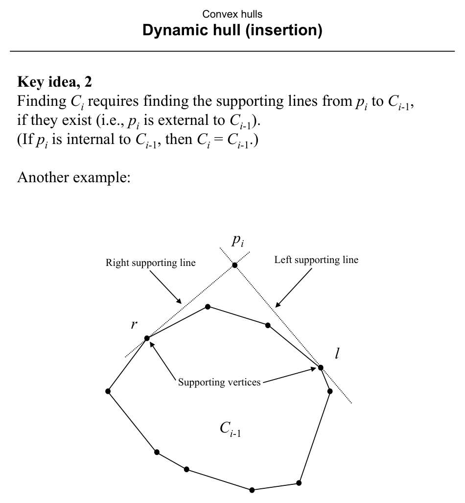
Same supporting-line picture for another configuration.
Slide 251: Algorithm outline
If \(p_i\) is external:
- Find supporting vertices \(\ell\) and \(r\) on \(C_{i-1}\).
- New hull boundary: \(p_i\) plus the chain of vertices of \(C_{i-1}\) from \(r\) to \(\ell\) (cyclic order), replacing the chain that becomes interior.
(Text alternates notation \(p/p_i\), \(C_{i-1}/C/P\).)
Slide 252: Classify a vertex \(v\) w.r.t. \(p_i\)
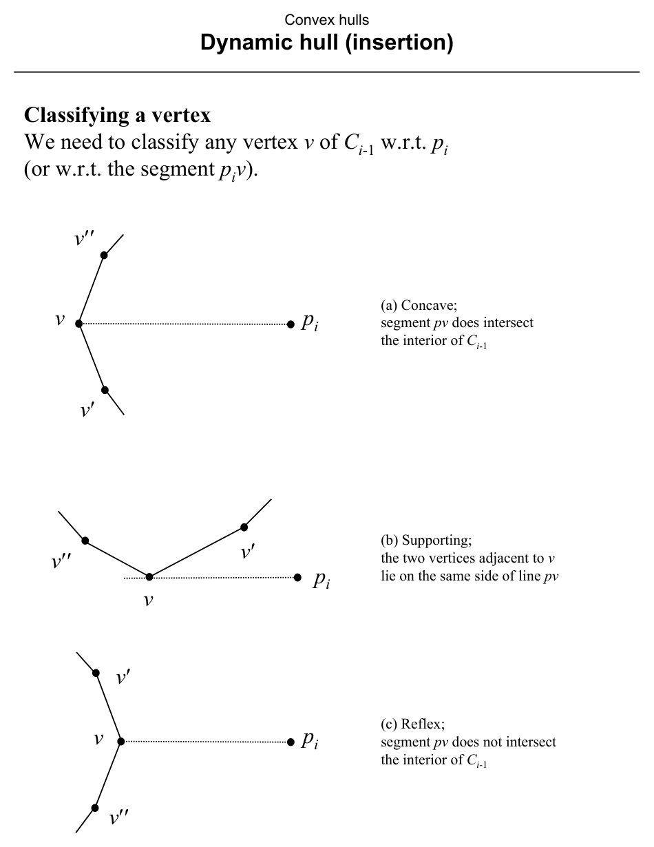
Relative to segment \(\overline{p_i v}\) and polygon \(C_{i-1}\):
- Concave (w.r.t. search): \(\overline{p_i v}\) meets the interior of \(C_{i-1}\).
- Supporting: neighbors of \(v\) on the hull lie on the same side of line \(p_i v\).
- Reflex (w.r.t. search): \(\overline{p_i v}\) does not meet the interior (advance the other way).
Slide 253: Walking to a supporting vertex
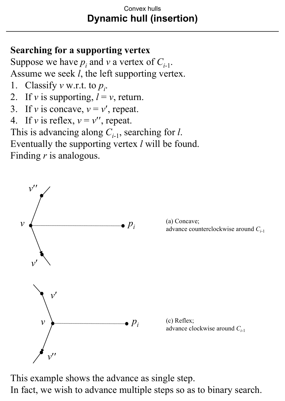
To find left supporting vertex starting from \(v\): classify \(v\); if supporting, done; if concave, step to \(v'\); if reflex, step to \(v''\). Binary search on the balanced tree refines this to \(O(\log N)\) instead of linear walk.
Slide 254: Required DS operations
Structure for vertices of \(C_{i-1}\) must support:
- SEARCH — locate supporting edges/vertices from \(p_i\).
- SPLIT — cut a cyclic vertex list.
- CONCATENATE / SPLICE — join lists.
- INSERT — place \(p_i\).
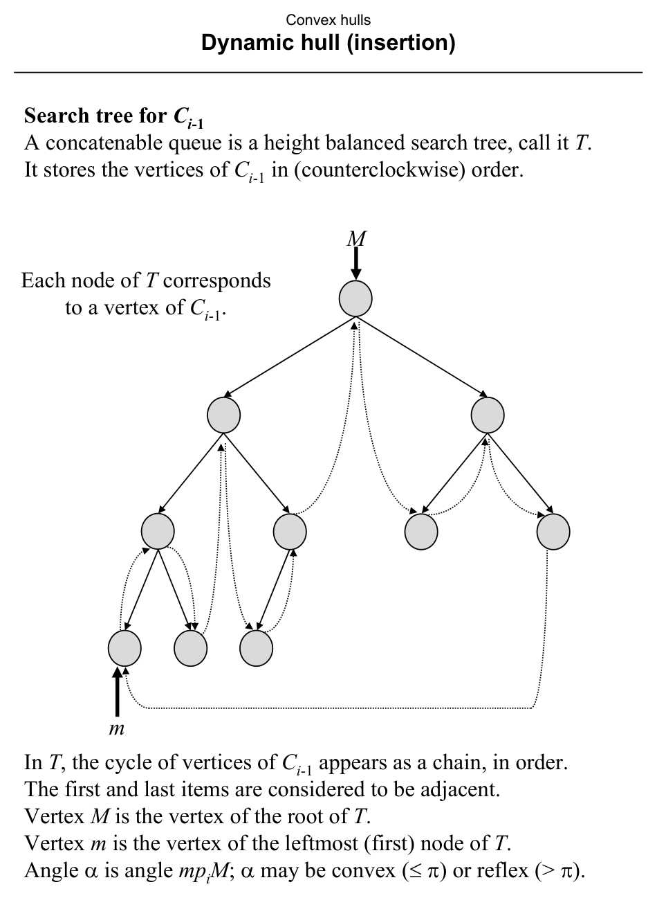
A concatenable queue (height-balanced search tree with threading) implements these in \(O(\log N)\) per operation (see Aho 1974, Reingold 1977). Thread links help access subtree minima in \(O(1)\) per recursive step.
Slide 255: Search tree \(T\) for \(C_{i-1}\)
Vertices of \(C_{i-1}\) in counterclockwise order appear as an in-order chain in balanced tree \(T\); first and last are adjacent on the hull cycle. Root stores vertex \(M\); leftmost leaf stores \(m\). Angle \(\alpha = \angle m\,p_i\,M\) may be convex (\(\le\pi\)) or reflex (\(>\pi\)).
Slides 256–257: Case analysis
Classifications of \(m\), \(M\) (concave / supporting / reflex) and whether \(\alpha\) is convex or reflex give 18 combinatorial patterns, collapsing to 8 distinct actions. Figure 3.16 (text p. 122) illustrates them; \(L(M)\) and \(R(M)\) denote vertex sequences in the left and right subtrees of the root.
Slide 258: Figure for cases
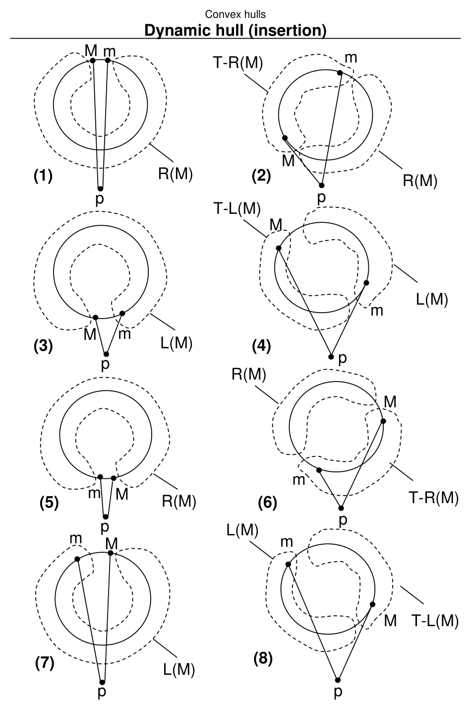
Slide 259: LEFTSEARCH (cases 2,4,6,8)
When \(\ell\) and \(r\) lie in different subtrees of the current root, recurse analogously in each subtree. Sketch:
procedure LEFTSEARCH(T)
  c ← ROOT(T)
  if line p_i c is supporting then return c
  else if c is reflex then T ← LTREE(c)
  else T ← RTREE(c)   /* c concave */
  endif
  return LEFTSEARCH(T)
endif
RIGHTSEARCH is symmetric.
Slide 260: Cases 1,3,5,7
Here \(\ell,r\) may be absent (\(p_i\) internal) or both lie in the same subtree (circled in Fig. 3.16). Recurse into that subtree until a case 2/4/6/8 node separates \(\ell\) and \(r\).
Slide 261: Cost of search
One root-to-leaf path locates the split point; then two downward paths find \(\ell\) and \(r\). Tree height \(O(\log N)\), \(O(1)\) work per node → \(O(\log N)\) per insertion search.
Slide 262: Splicing \(p_i\) in
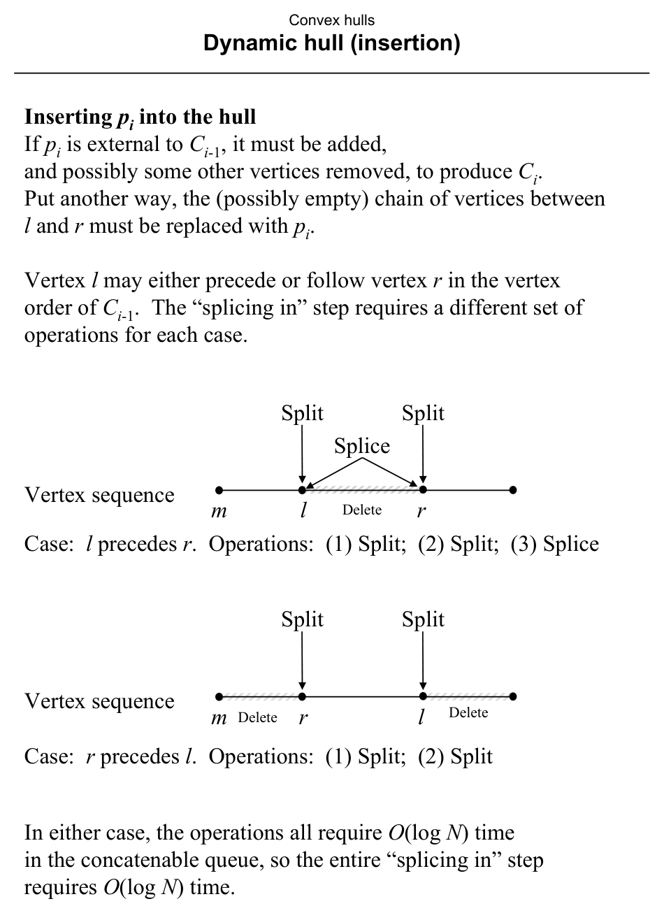
Replace the hull chain between \(\ell\) and \(r\) by \(p_i\) using split / splice / delete on the concatenable queue. Whether \(\ell\) precedes \(r\) or the reverse determines the exact sequence (one case: split + split; other: split + split + splice). Each operation \(O(\log N)\).
Slide 263: Analysis
Per insertion:
- \(O(\log N)\) — find \(\ell, r\).
- \(O(\log N)\) — splice in \(p_i\).
Total for \(N\) insertions: \(O(N \log N)\). Storage: \(O(N)\) for \(T\).
Recap
- On-line / real-time hull: after each insertion, maintain \(H(\{p_1,\ldots,p_i\})\); insertion-only dynamic hull generalizes to deletions later.
- External point: find left and right supporting vertices from \(p_i\) to the previous hull; splice out the chain between them and insert \(p_i\).
- Data structure: concatenable queue (balanced tree + threading) supports search, split, splice in \(O(\log N)\); case analysis on \((m,M,\alpha)\) guides binary search for supports.
- Total: \(O(N \log N)\) for \(N\) insertions, \(O(N)\) storage.